Approximating Binomial with Poisson
It is usually taught in statistics classes that Binomial probabilities can be approximated by Poisson probabilities, which are generally easier to calculate. This approximation is valid “when
In this post I’ll walk through a simple proof showing that the Poisson distribution is really just the Binomial with
Proof
The Binomial distribution describes the probability that there will be
Let
where
This is the rate of success. That’s the number of trials
Solving for
I then collect the constants (terms that don’t depend on
Now let’s take the limit of this right-hand side one term at a time.
- We start with the blue term
The
- Now we focus on the red term of (2)
Recall the definition of
Substituting it into our expression we get
- The third term of (2) is
Putting these together we can re-write (2) as
where
Casella and Berger (2002) provide a much shorter proof based on moment generating functions.
A natural question is how good is this approximation? It turns out it is quite good even for moderate
Code
A rule of thumb says for the approximation to be good:
“The sample size
should be equal to or larger than 20 and the probability of a single success, , should be smaller than or equal to 0.05. If > 100, the approximation is excellent if is also < 10.”
Let’s try a few scenarios. I have slightly modified the code from here.
# plots the pmfs of Binomial and Poisson
pl <- function(n, p, a, b) {

   clr <- rainbow(15)[ceiling(c(10.68978, 14.24863))]
   lambda <- n * p
   mx <- max(dbinom(a:b, n, p))

   plot(
      c(a:b, a:b),
      c(dbinom(a:b, n, p), dpois(a:b, lambda)),
      type = "n",
      main = paste("Poisson Approx. to Binomial, n=", n, ", p=", p, ", lambda=", lambda),
      ylab = "Probability",
      xlab = "x")
   points((a:b) - .15,
          dbinom(a:b, n, p),
          type = "h",
          col = clr[1],
          lwd = 10)
   points((a:b) + .15,
          dpois(a:b, lambda),
          type = "h",
          col = clr[2],
          lwd = 10)
   legend(b - 3.5, mx, legend = c("Binomial(x,n,p)", "Poisson(x,lambda)"), fill = clr, bg = "white")
}
I start with the recommendation:
pl(20, 0.05, 0, 10)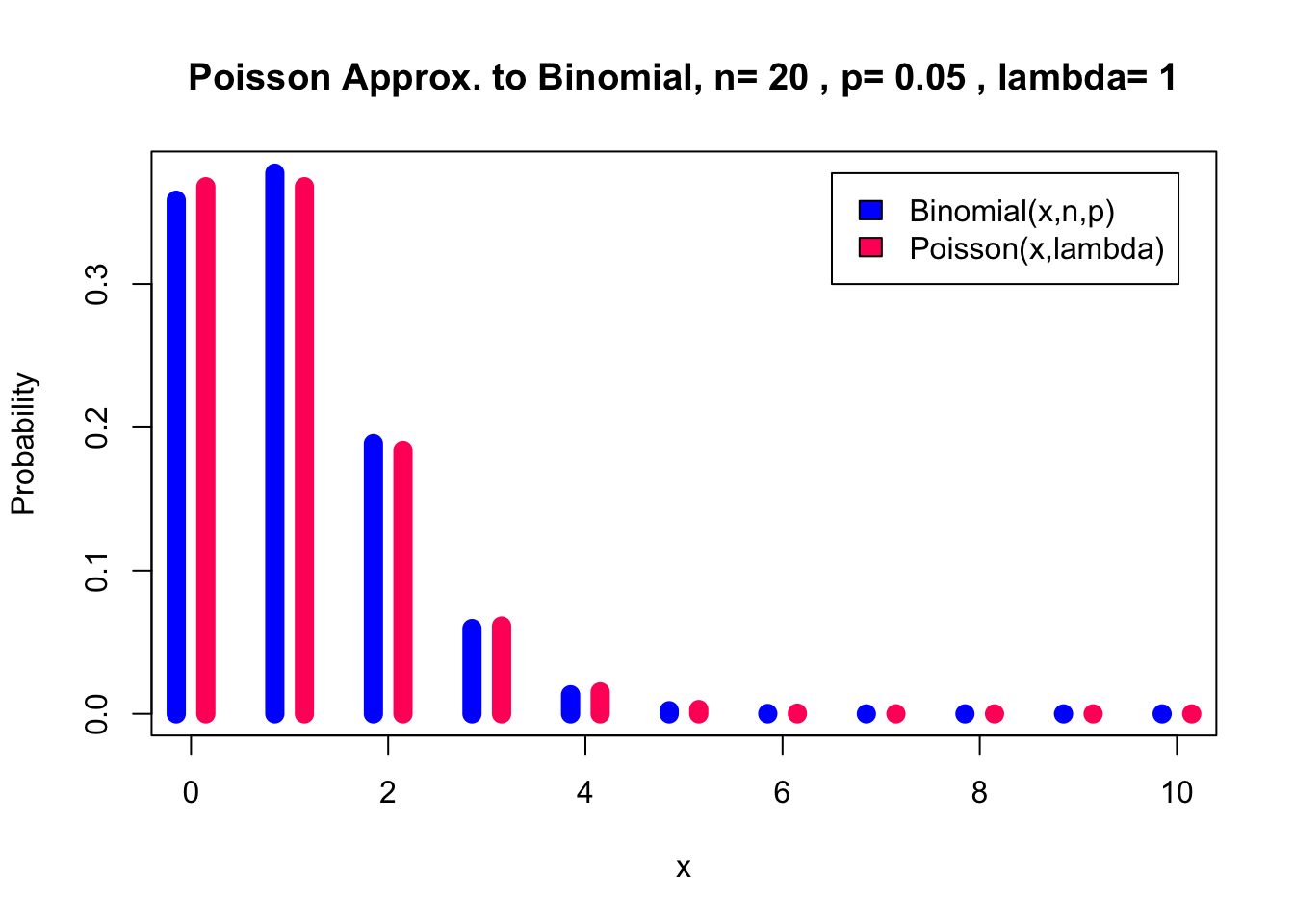
For
pl(10, 0.3, 0, 10)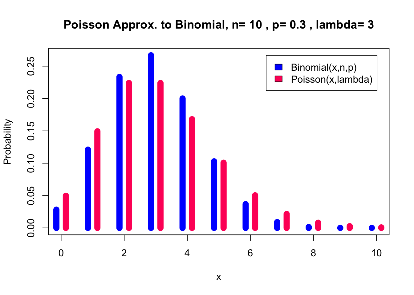
But if we increase
pl(100, 0.03, 0, 10)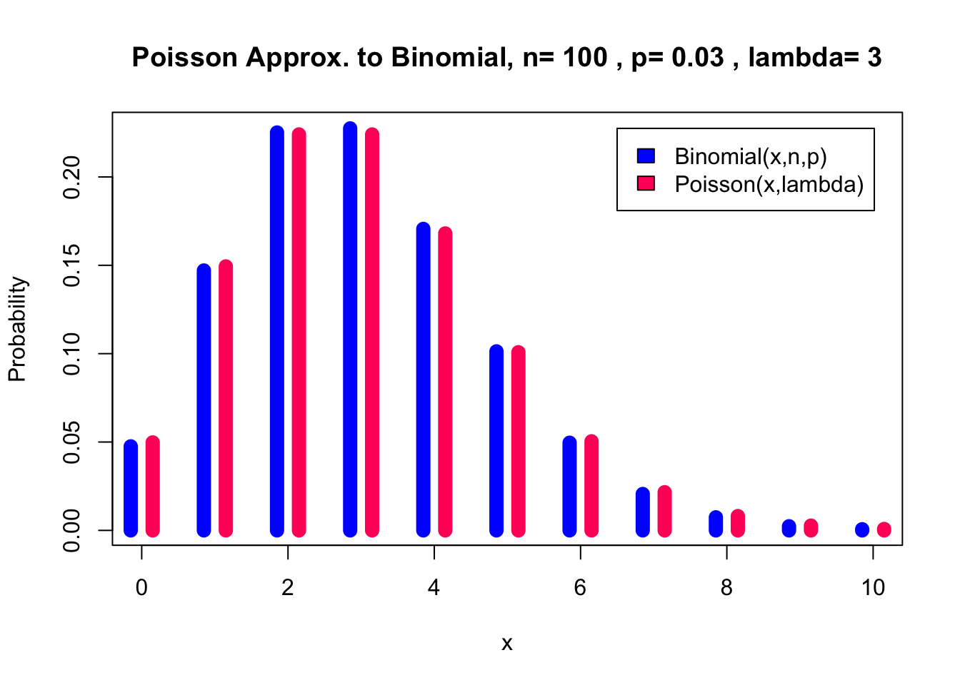 Lastly, for 1000 trials the distributions are indistinguishable.
pl(1000, 0.003, 0, 10)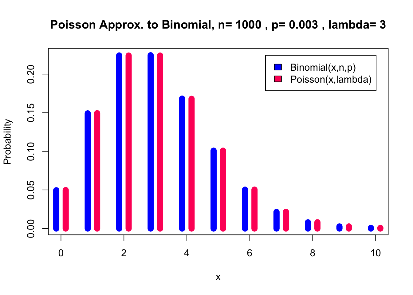
References
Casella, George, and Roger L Berger. 2002. Statistical Inference. Vol. 2. Duxbury Pacific Grove, CA.